Method for Estimating Time Series Data of COVID-19 Deaths using a Gumbel Model
Article Information
Furutani H1*, Hiroyasu T1, 2, Okuhara Y3
1AI x Humanity Research Center, Doshisha University, Kyoto, Japan
2Department of Biomedical Information, Doshisha University, Kyoto, Japan
3Medical School, Kochi University, Kochi, Japan
*Corresponding author: Hiroshi Furutani, AI x Humanity Research Center, Doshisha University, Kyoto, Japan
Received: 27 December 2021; Accepted: 04 January 2022; Published: 11 January 2022
Citation: Furutani H, Hiroyasu T, Okuhara Y. Method for Estimating Time Series Data of COVID-19 Deaths using a Gumbel Model. Archives of Clinical and Biomedical Research 6 (2022): 50-64.
View / Download Pdf Share at FacebookAbstract
The purpose of the present paper is to introduce a method for forecasting the daily number of COVID-19 associated deaths. We apply the Gumbel distribution function for the analysis of time series data of the first-wave outbreak. The Gumbel distribution function FG(t) has the property of having a mode (peak) point b, where FG(b)=1/2.718. The probability density function of FG(t) has a single-peaked and right-skewed form. Using this distribution, we can estimate the total number of deaths N, and forecast daily numbers in the decreasing phase. We study the early-stage data of Italy, Canada, Belgium, Switzerland, the Netherlands, Sweden, Germany, China, France, and the United Kingdom. The data of New York City and England are also analyzed. In general, the Gumbel distribution reasonably reproduces the time series data of daily counts. However, significant discrepancies between theory and data are observed for China, France, and Sweden. We re-analyze the data of these countries and the Netherlands using different approaches.
Keywords
COVID-19; Forecast; Extreme values; Gumbel distribution; Daily number of deaths
COVID-19 articles; Forecast articles; Extreme values articles; Gumbel distribution articles; Daily number of deaths articles
Article Details
1. Introduction
Coronaviruses are large, enveloped RNA viruses, the importance of which has been recognized through the identification of a newly emerged coronavirus as the causative agent of severe acute respiratory syndrome (SARS) [1]. The worldwide pandemic called COVID-19 is caused by the most recently discovered coronavirus, SARS-CoV-2, and is ``the third documented spillover of an animal coronavirus to humans in only three decades that has resulted in a major epidemic'' [2]. The 2003 outbreak of SARS had a case-fatality rate of approximately 10% (774 deaths), and MERS killed 34% of people with illness between 2012 and 2019 (2,494 deaths). While the case-fatality rate of COVID-19 is a few percent, the associated pandemic has caused many more deaths worldwide [3]. The international research community is currently fighting this global health crisis. There have been numerous efforts to develop mathematical methods in the field of epidemiology [4, 5]. Kermack and McKendrick developed a fundamental theory of epidemics called the SIR model, which is composed of three compartments: Susceptible S, Infected I, and Recovered/Removed R [6]. Their approach is one of the most frequently used mathematical models for analyzing epidemics. The SIR model is defined by coupled ordinary differential equations including a term of quadratic nonlinearity SI. They also showed that the SIR model can be reduced to a logistic model under natural assumptions. This logistic model was applied to the analysis of death counts for the 1905–1906 plague of the island of Bombay, and it was shown that the logistic distribution can fit the weekly number of deaths very well.

The application of the logistic model to the study of the COVID-19 outbreak has been reported by many researchers. In China, COVID-19 caused a great threat to the public health system from mid-January till mid-March 2020. Analysis with the standard logistic distribution model demonstrated that this simple function can summarize the outbreak dynamic of COVID-19 for 20 provinces in China excluding Hubei [7]. The cumulative number of cases was very well described by a logistic growth model with a coefficient of determination R2 greater than for all provinces. The logistic model was also applied to the analysis of the COVID-19 epidemic in Italy [8-11]. The analysis of severely infected people from 2020/2/24 to 2020/4/1 in Italy and its five regions demonstrated that the logistic growth curve reproduces these time series data very well [10]. However, most data after the peak are not included in this analysis. A similar analysis of the daily number of infected people was carried out using the data from 2020/2/27 to 2020/6/3 [11]. After a smoothing procedure, it was shown that the time series data have a right-skewed distribution. Since the logistic distribution is symmetric, the fitting by this model cannot reproduce the data reported for Italy. Therefore, the authors introduced a new method using a logistic equation called the stretched logistic equation with a time-dependent growth rate. This extended logistic function reproduced the data of the entire period very well.
In the first wave of a pandemic in many regions, the daily plot of reported deaths is single-peaked and skewed to the right. Time series data generally have three phases: (A) an exponential increase in the early stage, (B) an intermediate stage changing from increasing to decreasing, and (C) a slowly decreasing final stage. Taking into account the characteristics of COVID-19 data, the present study makes use of extreme value (EV) statistics to estimate the daily numbers for (C) and the total number of deaths from the data of (A) and (B). Extreme value theory provides methods by which to analyze the maximum (or minimum) value samples derived from distributions, such as normal or exponential distributions. Extreme value theory has been used in many fields to estimate the probability of rare events from observed data [14]. The Fisher-Tippett type I distribution [15], i.e., the Gumbel distribution, is a distribution of maximum (or minimum) values from the data of several distributions. The Gumbel function for maximum values has a right-skewed form, and that for minimum values has a left-skewed form.
The present study considers the Gumbel function for maximum values. The CDF of this function is given as
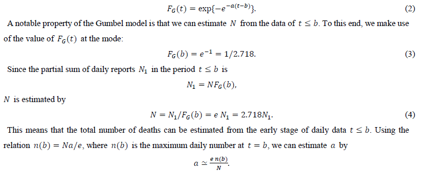
The proposed method is applied to the first-wave data of the COVID-19 daily number of deaths in Italy, Canada, Belgium, Switzerland, the Netherlands, Sweden, Germany, China, the United Kingdom, England and three of its regions, and New York City.
2. Methods
2.1 Dataset
The present study uses four datasets for the analysis of daily COVID-19 deaths.
Dataset A: For the analysis of data in Canada, France, Belgium, Netherlands, Germany, Italy, Switzerland, and China, we downloaded the dataset from the website of the European Center for Disease Prevention and Control
https://www.ecdc.europa.eu/en/publications-data/.
The dataset consists of historical data (to 14 December 2020) for the daily number of COVID-19 cases and deaths by country worldwide.
The file name is ``COVID-19-geographic-distribution-worldwide-2020-12-14.xlsx''(accessed on 2021/4/21).
- Dataset B: We downloaded the daily number of COVID-19 deaths from the official website of New York City https://www1.nyc.gov/site/doh/covid/covid-19/.
COVID-19 deaths are categorized as probable or confirmed.
Confirmed death: Death within 60 days of a positive molecular test.
Probable death: Cause of death on the health certificate is COVID-19 or similar, but a positive molecular test is not on record.
The file name is ``deaths-by-day.csv'' (accessed on 2021/5/15).
- Dataset C: We used the dataset of the official UK government website for data on coronavirus. https://www.coronavirus.data.gov.uk/details/deaths/ (accessed on 2021/4/22)
The downloaded files include (1) the number of deaths of people whose death certificate mentioned COVID-19 as one of the causes and (2) the daily number of deaths within 28 days of a positive test.
- Dataset D: The dataset of England NHS is downloaded for the analysis https://www.england.nhs.uk/statistics /statistical work areas/covid-19-daily-deaths/ (accessed on 2021/5/1).
This website contains the dataset of COVID-19 deaths in England and seven of its regions. The data of London and two regions are selected for the analysis. The present study treats the deaths of patients who have died in hospitals in England and have tested positive for COVID-19.
2.2 Gumbel model
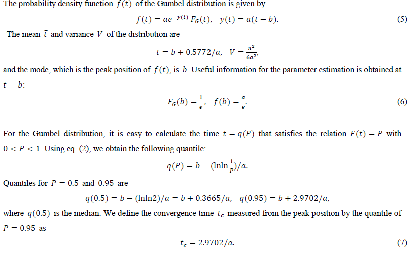
2.3 Estimation of daily and total numbers
This subsection describes the process for estimating the daily data and the total number. The date is indexed as t=0 when the first case was reported. Later, we will redefine the starting date for the convenience of comparing the data of different regions. We use the symmetric 7-day moving average n(t) as the daily data in this analysis:

where denotes the reported daily number. Note that includes the information of, dt+1,dt+2 and dt+3. In the process of calculations, note that, for the data of Switzerland, it is necessary to use the 9-day average because even data for the 7-day average fluctuate considerably around the trend line.
The accumulated number U(t) is calculated usingdi:

From U(t), we estimate the distribution function FG(t).
2.4 Forecasting of daily numbers
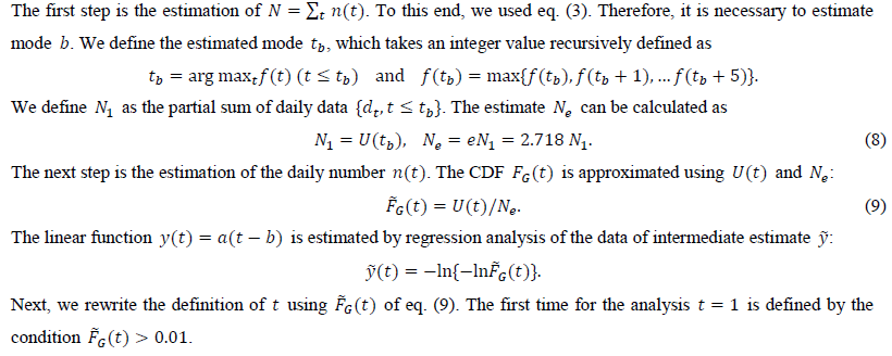
We calculate the estimate of y(t) from the intermediate estimate y using the regression analysis program. After performing a linear regression of the dependent variable and the independent variable t, we obtain two estimated parameters, a and b. The present study uses tmax points for the regression:

There is another way to estimate a. From eq. (6), we obtain an estimate of a as

3. Results
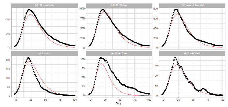
The present study analyzes the daily numbers and the total number of deaths in the first wave of the COVID-19 pandemic. We selected the data of ten countries: Italy, Canada, Belgium, Switzerland, the Netherlands, Sweden, France, Germany, China, and the United Kingdom. One city in the United States, New York City, was also used. We investigate the data of England and three of its regions, including London. All time series plots in the present study are single-peaked and skewed to the right, except for the data for China.
3.1 Results using dataset A
Table 1 shows a summary of the analysis using Dataset A.
|
date of t=1 |
tb |
Ne |
ye (t) |
tc |
|
|
Italy |
2020/3/9 |
23 |
31,508 |
0.06547 (t-23.93) |
45.37 |
|
Canada |
2020/4/2 |
33 |
10,009 |
0.04689 (t-32.56) |
63.34 |
|
Belgium |
2020/3/21 |
22 |
10,911 |
0.07010 (t-22.33) |
42.37 |
|
Switzerland |
2020/3/18 |
21 |
1,587 |
0.07799 (t-20.72) |
38.08 |
|
Netherlands |
2020/3/19 |
19 |
4,800 |
0.08214 (t-19.46) |
36.16 |
|
Sweden |
2020/3/20 |
26 |
3,961 |
0.05995 (t-27.39) |
49.54 |
|
Germany |
2020/3/24 |
26 |
11,172 |
0.06243 (t-25.27) |
47.58 |
|
China |
2020/1/26 |
22 |
4,529 |
0.06591 (t-23.12) |
45.06 |
|
France |
2020/3/19 |
20 |
24,223 |
0.06633 (t-23.94) |
44.78 |
Table 1: Summary of Gumbel analysis using Dataset A.
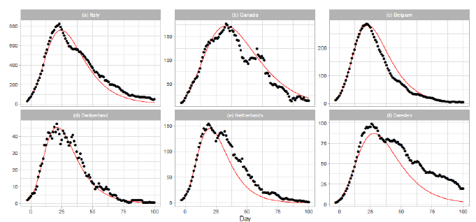
3.1.1 Italy, canada, belgium, and switzerland: The results of the Gumbel analysis for (a) Italy, (b) Canada, (c) Belgium, and (d) Switzerland are shown in Fig. 1. The number of data points used in the regression analysis is for these countries. The government of Italy extended the lockdown imposed on northern regions to the entire country on 2020/3/9, with containment measures including restrictions on travel and public gatherings [10]. The date 2020/3/9 corresponds to t=1 in Figure 1(a). In Canada, the first confirmed death was reported on 2020/3/8 [17]. The border was closed to non-citizens except travelers from the US on 2020/3/16. The border with the US was closed on 2020/3/22. Belgium reported the first confirmed death on 2020/3/10 [17]. The government of Belgium imposed a lockdown on 2020/3/17 (t=-3) with travel and gatherings prohibited and non-essential shops closed. The lockdown was extended until 2020/5/3 (t=44). Thus, the lockdown period of Belgium is shown in Figure 1(c). In Switzerland, the first COVID-19 death was reported on 2020/3/5. On 2020/3/13, the federal government closed all schools until 2020/4/4 and banned gatherings of more than 100 people. On 2020/3/16, the federal government declared the existence of an extraordinary situation. On 2020/3/20, the federal government announced that no complete lockdown would be implemented, but banned gatherings of more than 5 people.
3.1.2 The netherlands and sweden: The results of analysis for the Netherlands and Sweden are presented in Figs. 1(e) and 1(f). The number of data points used in the regression analysis is for the Netherlands and for Sweden. The theory estimates lower than reported values of daily death for both countries. In particular, this discrepancy is significant for Sweden. The Netherlands has taken a liberal policy course [18]. A mild lockdown was implemented with individual freedom and responsibility. Sweden has managed the pandemic with no lockdowns, less regulation, and more voluntary action. There has been much discussion on the policy of Sweden regarding the perspective of herd immunity [19].
Figure 1: Gumbel model estimation based on the time series data for (a) Italy, (b) Canada, (c) Belgium, (d) Switzerland, (e) the Netherlands, and (f) Sweden. Vertical axes show daily death counts. The reported data points are indicated by black points, and the theoretical estimations are indicated by solid red lines. The parameters of the Gumbel distribution are presented in Table 1. The reported data show the 7-day moving averages of daily numbers except for Switzerland. The reported data for Switzerland are the data for a -day moving average.
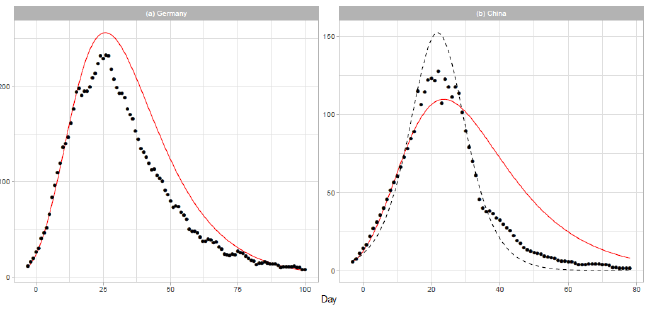
3.1.3 Germany and china: In Figure 2, we show the analysis of the daily COVID-19 deaths for Germany and China. The solid red lines show the theoretical results of the Gumbel model. The number of data points used in the regression analysis is for both countries. Germany is one of most affected countries in Europe. In March, Germany established several interventions to contain the virus spread, including the closure of schools and child day care facilities (2020/3/16-18) and a full lockdown with forced social distancing and closures of nonessential services (2020/3/23) [20]. Therefore, most of the data presented in Figure 2(a) were collected during the period of lockdown. In early December 2019, the Covid-19 outbreak began in the city of Wuhan, Hubei Province of China, and spread to other parts of China. On 2020/1/23,Wuhan was locked down. In the daily report of the dataset for China, the number of deaths on 2020/4/17 (t=83) is given as 1,290. We excluded this number from the analysis, considering that it may have been affected by a data gathering problem. In Figure 2(b), the result of logistic model estimation is presented by the dashed line. The parameters of the model are N = 3,345, a = 0.1827, and b = 21.32. The parameters a and b are obtained by a linear regression analysis using the 22 daily numbers of 1 ≤ t ≤ 22.
Figure 2: Gumbel model estimation based on the time series data for (a) Germany and (b) China. Vertical axes show daily death counts. The reported data are indicated by the points, and the theoretical estimations are indicated by the solid red lines. The points indicate 7-day moving averages of the reported data. The linear functions used for the Gumbel distributions are given in Table . For China, the logistic estimation is shown by the dashed line.
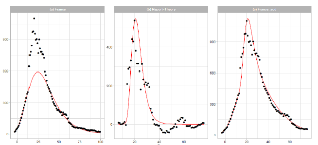
Figure 3: Gumbel model estimation based on the time series data for France: (a) the 7-day moving averages of the reported data (black points) and the Gumbel model estimation (solid red line), (b) difference of the reported data and the Gumbel model estimation (black points) and the second Gumbel model estimation (solid red line), and (c) the reported data ( black points) and the sum of the two Gumbel model estimations (solid red line). Vertical axes show daily death counts.
3.1.4 France: In Figure 3, we show the results of Gumbel analysis for France. In Figure 3(a), the solid red line indicates the theoretical estimation of the daily number of deaths with the model parameters presented in Table 1. The number of data used in the analysis is 15. Points show 7-day moving averages of the reported daily number of deaths. The government of France imposed a nationwide lockdown from 2020/3/17 to 2020/5/11 (-1 ≤ t ≤ 54 in Figure 3(a)) [17]. In contradiction with the implementation of severe restrictions, the government decided to allow municipal elections to proceed as scheduled starting on 2020/3/15, with minimal changes to voting procedures. Figure 3(b) shows the difference between the reported data and the theoretical estimation presented in Figure 3(a). The points are {reported data Gumbel model estimation}, and the solid red line is the Gumbel model fitting to the difference. The fitting parameters are Ne=6,000, a=0.2497, and b=20.24. The parameters and are calculated using data points within the region 14 ≤ t ≤ 33 . Figure 3(c) shows the reported data by points, and the sum of two Gumbel model estimations are shown by the solid red lines.
3.2 New york city
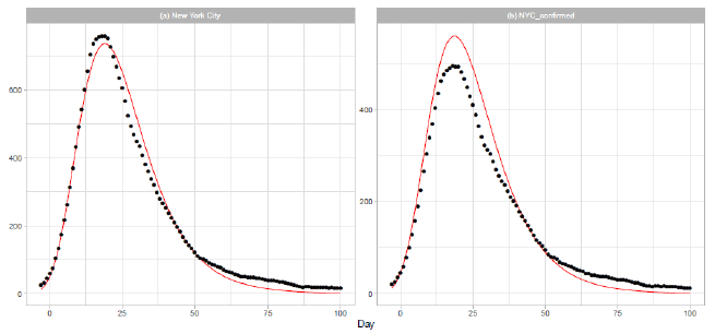
New York City (NYC) was an epicenter of the COVID-19 outbreak in the United States during spring [21]. On 2020/3/7, the governor declared a state of emergency in New York State. Th e mayor of NYC announced that all schools, bars, and restaurants in the city were to be closed from 2020/3/17, except for food takeout and delivery. In Figure 4, we report the results of our analysis of the daily data for NYC in Dataset B. The distribution parameters are presented in Table 2. Parameters and are obtained by a linear regression analysis using the 15 daily numbers of . Figure 4(a) shows the result of analysis of the sum of probable and confirmed deaths, and Figure 4(b) shows the result of analysis of the sum of confirmed deaths.
Figure 4: Gumbel model estimation based on the time series data for New York City: (a) probable and confirmed deaths, and (b) confirmed deaths. Vertical axes show daily death counts. The 7-day moving averages of daily data are indicated by the points, and the theoretical estimations are indicated by the solid red lines. Parameters for the estimation are given in Table 2.
|
date of t = 1 |
tb |
Ne |
yt |
||
|
New York City |
(a) reported |
2020/3/22 |
18 |
22,624 |
0.08862 (t-18.51) |
|
(b) confirmed |
2020/3/22 |
18 |
17,280 |
0.08830 (t-18.12) |
|
|
United Kingdom |
(a) certificate |
2020/3/20 |
22 |
46,510 |
0.06867 (t-23.46) |
|
(b) days |
2020/3/20 |
22 |
36,925 |
0.06852 (t-22.91) |
|
|
England |
(c) hospital |
2020/3/19 |
21 |
26,675 |
0.07048 (t-22.42) |
|
London |
(d) hospital |
2020/3/17 |
21 |
7,127 |
0.07292 (t-21.83) |
|
North East |
(d) hospital |
2020/3/22 |
17 |
2,582 |
0.09262 (t-17.84) |
|
South West |
(d) hospital |
2020/3/20 |
20 |
1,166 |
0.07204 (t-21.67) |
Table 2: Parameters of Gumbel estimation for analyzing Datasets B, C, and D.
Figure 5: Gumbel model estimation based on the time series data for the United Kingdom: (a) the United Kingdom, death certificates, (b) the United Kingdom, deaths within days of the first positive test, (c) England, (d) London, (e) North East and Yorkshire, and (f) South West. Vertical axes show daily death counts. The 7-day moving averages of the reported data are indicated by the points, and the theoretical estimations are indicated by the solid red lines. Parameters for the estimation are given in Table 2.
3.3 United kingdom
On 2020/3/23, the United Kingdom Government imposed the instruction to stay at home, and people were allowed to leave their home for very limited purposes. The government closed all shops selling nonessential goods, stopped all gatherings of more than two people in public, and banned all social events. The results of Gumbel analysis for the United Kingdom are shown in Figure 5. The number of data points used in the regression analysis is 15. The daily numbers of Dataset C are used in Figs. 5(a) and 5(b), and those of Dataset D are used in Figures 5(c), 5(d), 5(e), and 5(f). Figure 5(a) shows the results for daily counts of deaths of people whose death certificate mentioned COVID-19 as one of the causes, and Fig. 5(b) shows the results for daily counts of deaths of people who had had a positive test result for COVID-19 and died within days of the first positive test. We downloaded daily records from the database of the National Health Service (NHS) of England for the analysis of England and three regions of the NHS of England: London, North East and Yorkshire, and South West. The dataset includes information on deaths of patients who have died in hospitals in England.
3.4 Different approach for the netherlands and sweden
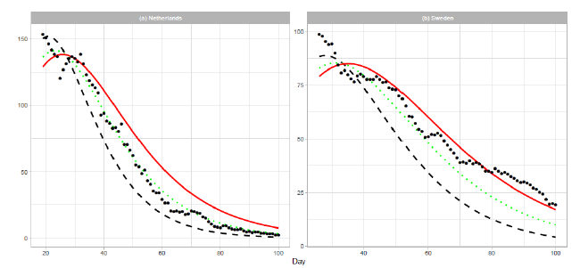
An optimistic estimation or underestimation may cause the risk of overwhelming health services. The estimations for the Netherlands and Sweden in Figure 1 are such cases. The reported data are far larger than the estimated deaths after . Therefore, we show an approach to modify estimation parameters after the date of the peak. If reported numbers are larger than those estimated by an epidemiologic model, we have to modify the initial estimation parameters. First, we replace the number of total deaths with . For simplicity, we use three cases of : , , and . For each parameter , we calculate the Gumbel parameters and by linear regression. For this analysis, we use the cumulative number in the period . Thus, the proposed method gives the estimation for . Table 3 presents the renewed Gumbel parameters for two countries. Figure 6 shows the results of new estimation. The result for the Netherlands in Figure 6(a) shows that the estimated number of daily deaths decreases along the line of . In Figure 6(b), the reported data for Sweden decrease between the lines of and and finally decrease more slowly than the estimation of . The reported data for Sweden indicate an increase in daily cases.
|
Ne' |
ye (t) |
|
|
The Netherlands |
1.1 Ne |
0.07833 (t-20.30) |
|
1.3 Ne |
0.06164 (t-22.68) |
|
|
1.5 Ne |
0.05228 (t-25.27) |
|
|
Sweden |
1.1 Ne |
0.05548 (t-27.32) |
|
1.3 Ne |
0.04510 (t-30.68) |
|
|
1.5 Ne |
0.03891 (t-34.16) |
Table 3: Parameters of Gumbel estimation for renewed analysis of the Netherlands and Sweden.
Figure 6: Renewed Gumbel model estimation based on the time series data of (a) the Netherlands and (b) Sweden. Vertical axes show daily death counts. The reported data are indicated by the points, and the theoretical estimations are indicated by dashed lines for , dotted lines for , and solid red lines for 1.5Ne.
4. Discussion
Some approaches use the phenomenological model, initially assuming a certain type of distribution function in data analysis. The most popular approach is an exponential distribution, the CDF of which is defined as

In the epidemiology analysis, many studies suggest that this model can reasonably reproduce the data in the decreasing phase (e.g., [5]). The logistic distribution FL(t) has been also applied in the field of epidemiology, as shown in the present paper. The important point is that the logistic model is derived from the SIR model with very natural assumptions [22]. Thus, this distribution has the background of a dynamical model of infection. For large t, the logistic distribution is approximated by the following exponential distribution:

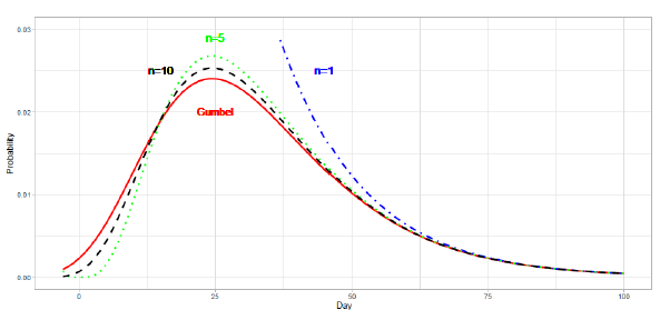
The third candidate is the Gumbel distribution. There are two types of Gumbel functions: the Gumbel function for maximum values and the Gumbel function for minimum values. The present study used the Gumbel function for maximum values. In a similar way as the logistic distribution, the Gumbel distribution approaches the exponential distribution for large t
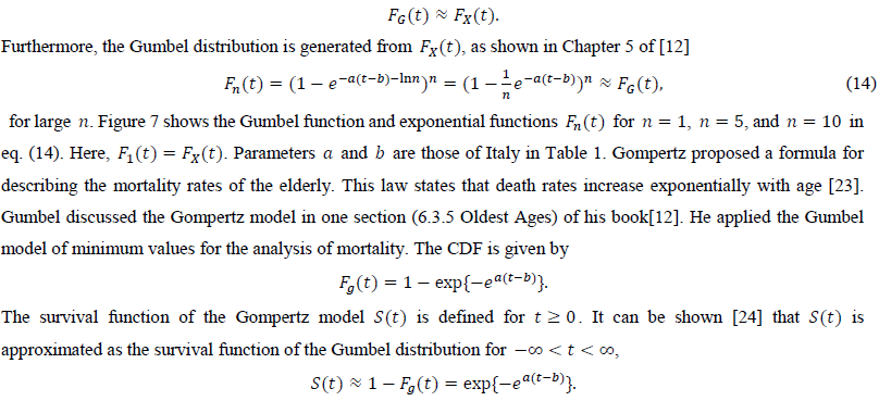
There are theoretical efforts to derive the Gumbel distribution of the smallest values to explain the phenomena of exponentially increasing mortality. Abernethy (1979) applied EV theory to this problem [25]. Their study used an analogy between the death of an organism and the failure of a multicomponent system and mathematically derived this type of Gumbel distribution. We hope that this line of approach can explain the applicability of the Gumbel distribution of maximum values to pandemic data.
The present study demonstrates the advantage of the EV theory for investigating time series data of deaths in pandemic outbreaks. We make use of one class of Gumbel distribution for the extremes of maximum values. The Gumbel distribution provides a means of extrapolation in time with theoretical justification by the EV theory and can be used to estimate the data in the decreasing phase from the data in the exponentially increasing phase. The Gumbel distribution reproduces the time series data of daily counts in many regions. However, notable discrepancies between estimation and reported data are observed for China, France, and Sweden. Therefore, we try to analyze the data of these countries under different approaches. In many regions, it is reported that the outbreak of a second wave of the pandemic began before the first wave of COVID-19 converged to a final stage [26]. We carried out calculations for the first wave data of the United States using Dataset A. The estimated total number of deaths is approximately . However, the second wave of the pandemic began during the decreasing phase of the first wave, so we cannot compare the time series of reported data and theoretical estimation for the entire period. We have designed a tool for analyzing the first and second waves of a pandemic simultaneously and intend to report this tool in the future.
Author Contributions
The present study was conducted equally by the authors. H.F. wrote the initial manuscript.
Competing Interests
The authors declare no competing interests.
Funding
This research did not receive any specific grant from funding agencies in the public, commercial or not-for-profit sectors.
References
- Masters PS. The molecular biology of coronaviruses. Virus Res 66 (2006): 193-292.
- V'kovski P, Kratzel A, Steiner S, Stadler H, Thiel V. Coronavirus biology and replication: implications for SARS-Cov-2. Rev. Microbiol (2020): 1-16.
- Mahase E. Coronavirus: covid-19 has killed more people than SARS and MERS combined, despite lower case fatality. BMJ 368 (2020).
- Brauer F. Compartmental models in epidemiology. In: Mathematical Epidemiology. Lecture Notes in Mathematics 1945 (2008): 19-79.
- Chowell G, Sattenspiel L, Bansal S, Viboud C. Mathematical models to characterize early epidemic growth: A review. Life Rev 18 (2016): 66-97.
- Kermack WO, McKendrick AG. A contribution to the mathematical theory of epidemics. Roy. Soc. London 115 (1927): 700-721.
- Zou Y, Pan S, Zhao P, Lei Han, Xiaoxiang Wang, Lia Hemerik, et al. Outbreak analysis with a logistic growth model shows COVID-19 suppression dynamics in China PLoS ONE 15 (2020): e0235247.
- Postnikov E B. Estimation of COVID-19 dynamics ``on a back-of-envelope'': Does the simplest SIR model provide quantitative parameters and predictions?. Chaos Solitons Fractals 135 (2020): 109841.
- Efim Pelinovsky, Andrey Kurkin, Oxana Kurkina, Maria Kokoulina, Anastasia Epifanovaa. Logistic equation and COVID-19. Chaos Solitons Fractals 140 (2020): 110241.
- Gabriele Martelloni, Gianluca Martelloni. Analysis of the evolution of the Sars-Cov-2 in Italy, the role of the asymptomatics and the success of Logistic model. Chaos Solitons Fractals 140 (2020): 110150.
- Consolini G, Materassi M. A stretched logistic equation for pandemic spreading. Chaos Solitons Fractals 140 (2020): 110113.
- Gumbel EJ. Statistics of Extremes, Columbia University Press, New York (1958).
- Coles S. An Introduction to Statistical Modeling of Extreme Values, Springer-Verlag, London (2001).
- Asadi ZS, Melchers RE. Extreme value statistics for pitting corrosion of old underground cast iron pipes. Eng. Syst. Saf. 162 (2017): 64-71.
- Fisher RA, Tippett LHC. Limiting forms of the frequency distributions of the largest or smallest numbers of a sample. Cambridge Phil. Soc. 24 (1928): 180-190.
- Carter DJT, Challenor PG. Methods of fitting the Fisher-Tippett type extreme value distribution. Ocean Engng 10 (1983): 191-199.
- Desson Z, Weller E, McMeekin P, Ammi M. An analysis of the policy responses to the COVID-19 pandemic in France, Belgium and Canada. Health Policy Technol 9 (2020): 430-446.
- Hoekman LM, Smits MMV, Koolman X. The Dutch COVID-19 approach: Regional differences in a small country. Health Policy Technol 9 (2020): 613-622.
- Jones D, Helmreich S. A history of herd immunity. Lancet 396 (2020): 810-811.
- Wieland T. A phenomenological approach to assessing the effectiveness of COVID-19 related nonpharmaceutical interventions in Germany. Sci. 131 (2020): 104924.
- Ana S Gonzalez-Reiche, Matthew M Hernandez, Mitchell J Sullivan, Brianne Ciferri, Hala Alshammary, Ajay Obla, et al. Introductions and early spread of SARS-Cov-2 in the New York City area. Science 369 (2020): 297-301.
- Barlow NS, Weinstein SJ. Accurate closed-form solution of the SIR epidemic model. Physica D 408 (2020): 132540.
- Gompertz B. On the nature of the function expressive of the law of human mortality, and on a new method of determining the value of life contingencies. Trans. R. Soc. 115 (1825): 513-585.
- Pflaumer P. Life table forecasting with the Gompertz distribution. JSM Proc. Alexandria, VA (2007): 3564-3571.
- Abernethy JD. The exponential increase in mortality rate with age attributed to wearing-out of biological components. Theor. Biol. 80 (1979): 333-354.
- Cacciapaglia G, Cot C, Sannino F. Second wave COVID-19 pandemic in Europe: A temporal playbook. Rep. 10 (2020): 15514.

